

Quadratic image projection
Earlier articles in this series on quick image scaling have presented algorithms to scale linearly, meaning that the resampling is uniform over the entire image. The effect is that of zooming into an image or zooming out of an image. When you want to mimic the effect of rotating the source image around its vertical axis, you must apply non-linear scaling to simulate the perspective foreshortening in the output image (the "projection"). This article analyses the foreshortening effect and presents an algorithm that approximates it. The first article in this series showed how Bresenham's line drawing algorithm was easily adapted to resample images. Here, I implement an adapted "Bresenham" algorithm that resamples along a quadratic curve (a parabola).
A common thread in the articles in this series is the term "approximation" and a justification why an approximation is advantageous to "the real thing". The smooth Bresenham algorithm of the first article is an approximation of linear interpolation and the article argues that it produces equivalent quality at a much reduced (performance) cost; the second article uses an approximate colour distance metric because it is faster and precision does not matter —the metric is just a hint for the direction of the interpolation; the third article is about calculating approximate averages of colours and it claims that the commonly used calculation method is already an approximation and that loosing one bit of precision weighs out against a significant gain in performance. This article, instead of following the true curve of the perspective foreshortening, approximates it with a quadratic curve and it starts by justifying that compromise.
As before, the algorithms that I present in this article needs to do its work in real-time. It has to be quick. A straight-forward implementation of the perspective projection requires a few multiplies and a divide per pixel. Multiply and, especially, divide instructions are relatively slow instructions; you wouldn't want to do them for every pixel. Also, the arithmetic must be done in floating point and floating point precision is finite. That is, floating point arithmetic is, at best, imprecise. When plotting a curve, being one pixel off due to an accumulated error of imprecise calculations isn't too bad. However, when you use the position on the curve to fetch a pixel from a source image, an off-by-one error might cause a pixel read beyond the bounds of the source image and result in a memory access violation. An implementation of perspective image scaling that uses floating point arithmetic must be carefully implemented to avoid such off-by-one errors.
The first article in this series mentioned a second algorithm by
Bresenham, one that approximates elliptical arcs. Actually, the same
transformation and algorithmic reasoning can be applied to any conic section.
The perspective foreshortening curve is a hyperbola and a hyperbola is, like
a circle, an ellipse and a parabola, a conic section. In other words, it is
possible to calculate the foreshortening curve with only integer arithmetic
and with only addition and subtraction. The general equation of a conic section
being
Ax2 + Bx + Cxy + Dy + Ey2 + F = 0
the book "Computer Graphics: Principles and Practice"
contains an (incomplete) implementation of an algorithm that can plot any conic
section, but limited to integer values of A, B, C, D, E and F. For the
foreshortening curve, support for fractional values in the parameters is a
requirement. Judging from the size and the complexity that the routine in "Computer Graphics" already has and the amount of complexity
that needs to be added to make it suitable for our purposes, I feel that it is
not worth the effort, in view of the marginal improvement of quality that it
would give.
The previous sentence may have raised eyebrows. In his paper on perspective texture mapping Dr. Smith argues that a polynomial (such as a parabola) cannot be sufficiently accurate in all cases to pass for a hyperbola. Chris Hecker also mentions the inaccuracy of the quadratic curve as a disadvantage in its use for perspective mapping in the fourth installment of his series on perspective texture mapping. With inaccuracy is meant that, if you use a quadratic curve as the basis for foreshortening, your images will have the wrong perspective. The importance of accuracy should not be overvalued, however. A perspective image is already an illusion (of a 3-D scene) and approximate foreshortening is sufficient to raise this illusion. Most of the images that we look at, be it renaissance paintings, photographs or rendered pictures, have inaccurate perspective, not necessarily because of the images themselves but because they are usually viewed from the wrong viewpoint. Every photograph, rendering or perspective drawing contains an implicit "projection point" from which the picture should be viewed for accurate perspective; for photographs this projection point is of course related to the focal length of the camera lens, and for rendered images it is related to the virtual camera position relative to the projection surface. Yet, photographs, movies, paintings, billboards and computer screens are viewed from many angles and many distances and all except one create the wrong perspective —which is why I claim that the need for accuracy in perspective should not be overrated. The importance of accuracy should not be undervalued either. If the deviation from the true foreshortening curve becomes too big, straight lines in the original scene may come out curved in the projection.
Quadratic Bresenham
In 1965 J.E. Bresenham published an algorithm to approximate line segments on a grid of discrete values and in 1977 he published another algorithm to approximate circular and elliptical arcs. Despite the similar construct —only integer addition and subtraction and a "decision" variable that is updated in every iteration, these two algorithms are very different. It turns out that the first algorithm can be extended to approximate any polynomial and that the second algorithm can basically draw any conic section. A parabola is both a polynomial and a conic section. I am basing my quadratic image scaling routine on Bresenham's first algorithm.
Bresenham's line drawing algorithm expresses the amount to add to the y coordinate at every next step on the x-axis as a fraction, and then keeps the (accumulated) fractional part of the summation separate from the integer part —and it updates the both the fractional and integer parts as soon as the fractional part exceeds unity. This algorithm is one that handles fractions and accumulated fractions in an efficient way, using the absolute precision of integer arithmetic.
Bresenham's second algorithm starts with the knowledge which two y-coordinates are the closest to the actual curve at the next step along the x-axis; this knowledge is derived from the slope of the curve at that point. Then, it reformulates the equation of the curve to express the difference between the real "y" value of the curve and both of the selected y-coordinates, and ends by choosing the nearest pixel (i.e., the minimum distance). All of this is folded into a new set of equations that directly update the criterion for selecting either of the two y candidates, so the real "y" coordinate on the curve never needs to be calculated. The gain of the algorithm is that multiplications and divides have vanished from the new equations. Bresenham's ellipse drawing algorithm can only cope with integer radii, however.
The general equation for the quadratic curve is:
y = A·x2 + B·x + Cwhere x is a coordinate along the horizontal axis and y a coordinate along the vertical axis in a two-dimensional plane. It simplifies the forward differencing equations when rewriting the equation to:
y = A·(x2 + C) + B·(x + C)(with different constants A, B and C). For our purpose of using the quadratic curve equation for a projection, it is convenient to rename y to u and x to x' (see also figure 1). Also, I introduce a new symbol, p, which is x'+C. With these substitutions, the above equation becomes:
u = A·p2 + B·p
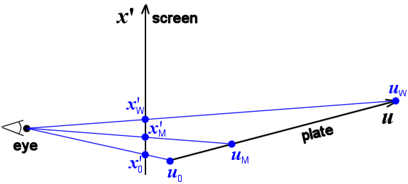
Figure 1: coordinate systems, nomenclature
Like was the case for the line equation, the first step is to rewrite the
equation as a forward differencing equation, where pi+1 is pi+1:
ui+1 = A·pi+12 + B·pi+1
ui+1 = A·(pi+1)2 + B·(pi+1)
ui+1 = A·pi2 + 2·A·pi + A + B·pi + B
ui+1 = ui + 2·A·pi + A + B
The increment for every iteration, "2·A·pi + A + B", can be further reduced by the use of second order differences. If we replace the term by the symbol du, then:
dui = 2·A·pi + A + Bwhere 2·A is a constant —we might call it ddu. This gives us [1]:
dui+1 = 2·A·pi+1 + A + B
dui+1 = 2·A·(pi+1) + A + B
dui+1 = 2·A·xi + 2·A + A + B
dui+1 = dui + 2·A
ui+1 = ui + dui
dui+1 = dui + ddu
Before proceeding with an implementation, let me present how the quadratic curve relates to perspective image projecting. In this context, I will use the terminology of texture mapping. The source image can be seen as a texture that is mapped to a rectangular surface in 3-D space. The coordinates of a pixel in the source image (called a "texel", for texture element, in the field of texture mapping) are denoted with the symbol pair (u,v). The coordinates in 3-D space are denoted with (x,y,z) and the screen coordinates are (x',y'). Figure 1 is a top view of a scene with the axis systems. So, basically, one wants to map from (x',y') to (u,v). Due to how CPU caches work, it gives best performance to loop over x' in the inner loop of the algorithm and have an outer loop over y'. Equation [1] expresses how y changes if x is incremented by one. In the image projection, we want to know how both u and v must be adjusted when x' increases by 1. That is, there are two quadratic curves being followed in parallel, one for u and one for v.
Pseudo-code for the algorithm is below. The pixels of the source image are represented by the two-dimensional array "sourceimage", and the output is the two-dimensional array "displaybuffer". The "integer" function returns the integer part of a (fractional) value.
calculate y_start and y_end
LOOP y' FROM y_start TO y_end
    calculate x_start and x_end
    calculate du, ddu, dv and ddv
    LOOP x' FROM x_start TO x_end
        displaybuffer[x', y'] = sourceimage[integer(u), integer(v)]
        x' = x' + 1
        u  = u + du
        v  = v + dv
        du = du + ddu
        dv = dv + ddv
    END LOOP
    y' = y' + 1
END LOOP
The pseudo-code assumes that the variables u, v, du, dv, ddu and ddv can hold fractional values. With Bresenham's technique, as outlined in "Image scaling with Bresenham", we separate each fractional value into a "whole" part and a fractional part, where the the fractional part is represented as a quotient of two integer numbers. In other words, each fractional value is represented by three integer values.
Returning to the parabola equation, what I have skipped so far is the calculation of the parameters of the parabola —the values of A, B and C. A parabola can be specified by three points, meaning that if we calculate the values for three (x',u) tuples we can derive the values of A B and C for a parabola that runs through these three points. The idea is to calculate three points on each scan line accurately, with the correct perspective equation, and to approximate all the other points. The first decision to make is exactly which three points to use. The start and end points on a scan line of the projected image are obvious candidates for two of the three required points. For the third point, I selected the point halfway the start and end points in the projected image. In my experience, this gives a better approximation of the perspective hyperbola than the point halfway the source image, which is usually suggested (see, for example, "Perspective Texture Mapping, Part 4").
I will sidestep the issue how to calculate a value for x' given u, or a value for u given x', and simply assume that by some means I have calculated the x' values for u=0 and u=width (of the scan line) —these are the tuples (x'0,u0) and (x'W,uW) in figure 1. The third tuple is (x'M,uM), where x'M=(x'0+x'W)/2 Once I have these tuples, it takes some tedious, but simple, algebra to come to the following equations:


Recall that pi is (x'i + C). As C is -x'0, p0 is zero and pW is (x'W - x'0).
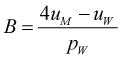
The equation to calculate A depends on the value of B being known; that is, you must calculate B before calculating A. Furthermore, the equation for B is the only equation that refers to the tuple (x'M,uM). In fact, it only refers to uM because x'M was replaced by (x'0+x'W)/2 and the equation was subsequently simplified. The effect of these properties is that the first equation calculates the value of A so that the parabola runs through the start and end points, whatever the value of B might be. This allows us to tweak the value of B, and still have a curve that runs through the start and end points of the source and destination scan lines.
Tweaking B is occasionally necesary to avoid overshoot. When the perspective foreshortening exceeds a certain limit, the approximating parabola reaches a maximum or minimum between the start and end points. In that situation, the u value (temporarily) exceeds either u0 or uW, see figure 2 for an example. Such an overshoot must be avoided, because we cannot read beyond the bounds of the source picture. The fix is to restrict B to a range where no overshoot occurs. For this, we have to analyse the derivative of the quadratic equation. A maximum or minimum between the start and end points occurs when the derivative switches sign halfway the trajectory. What we want, for our purposes, is either a monotomically increasing curve or a monotomically decreasing curve —which of the two depends on whether pW is greater or smaller than 0.
Figure 2: Parabola exceeding bounds
When pW is greater 0, the curve must be monotomically increasing, meaning that at the start of the curve the value of the derivative must be positive (zero or above) and at the end of the curve the derivative must still be positive. The parabola has only one "bent", so if the slope is increasing at both extrema, it must have been increasing all the way. The derivative of the equation:
u = A·p2 + B·pis:
δu = 2·A·p + Band we want to make sure that δu is greater than or equal to zero at both p0 and pW. As p0 = 0, the lower bound for B is zero. To calculate the upper bound, I substitute A with its equivalent fraction. After simplification the upper bound becomes:
When also substituting B with its equation, both bounds can be expressed in to the criterion:

or even simpler:
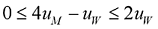
There is a caveat in this analysis, knowing that uM and uW are integers. In an extreme case, it can happen that no integer for uM exists that complies with both bounds: if uW is 1, for instance, any value for uM exceeds either bound. I have chosen to give up on these cases and revert linear interpolation, by forcing A to zero.
The implementation of the quadratic projection is in listing 1. The loop in function is very similar to that of the pseudo-code above. To make working with fractional values, with Bresenhams's method, easier, I implemented a primitive "Fractional" class. This is not a general purpose class for working with fractions: it does not even store the denominator of the fraction, but simply assumes that all fractions have the same denominator. The C/C++ language leaves the direction of the truncation for integer division "implementation defined" if either operand is negative. Since, I depend on the modulus (of a quotient) to be a positive value, I explicitly test for negative results and correct them.
There are hidden multiplications in the pseudo-code for the algorithm. An image is usually represented (in memory) as a two-dimensional array of pixels, and reading a pixel is an array indexing operation. To calculate the memory address associated with an index, the compiler multiplies the index by the size of one element or the size of one row of elements. So reading from a two-dimensional array masquerades two multiplications. As multiplications are relatively slow operations, removing them has some merit, especially because it is, conceptually, quite simple: pre-multiply u, du and ddu by the size of a pixel and pre-multiply v, dv, and ddv by the size of a scan line. Only the integer parts of the fractions should be scaled; the fractional parts stay as they are.
Projecting an image
I implemented a program to rotate an image over two angles and display the perspective projection of this image. To get the quadratic Bresenham algorithm started, we need to calculate the mapping of three points, as described earlier. To get those three points, we must first project the four vertices of the original flat rectangle of the image in order to get the outline of the projected image. Then, we can find the start and end points of all scan lines that run through the projection and calculate the middle point. Finally, we need to have a way to calculate a mapping from the projected coordinates back to coordinates relative to the original image. So there is some ground to cover, still.
Rotating a plane is usually done via transformation matrices and homogeneous vectors. Here, however, I have opted for for a simple calculation of a rotation over the x and y axes, instead of going for a general matrix transformation approach. I call the rotated image in 3-D space the plate (in the sense of a glass plate from the early days of photography). A plane is infinite and shapeless, but a plate is rectangular and bounded to the size of the image. I define a plate by specifying the (x,y,z) coordinates of its four vertices; this carries a bit redundancy, but it is convenient.
The next step is to project the plate on a 2-D screen. The perspective equation is:
x' = D·x / (z-D)where x and z are the coordinates of a pixel in 3-D space and D is the distance of the eye to the screen. I have put the origin of the axis system at the screen with the positive z-axis pointing away from the viewer. This means that D is a negative value. Mapping the four vertices of the plate results in a 2-D quadrangle that is the outline of the perspective projection of the plate.
The actual projection is done with quadratic Bresenham that runs over horizontal scan lines in 2-D "screen" space. We can now easily find the extents of the scan lines by finding the intersection points of a horizontal line with the projected plate. That done, we have x'0 and x'W, and x'M is easy to come up with. We can calculate the parameters of the parabola once we calculate the mapping of x'0 x'M and x'W to u0, uM and uW respectively. To map from x' to x to u, we need the inverse of the perspective projection. I have used techniques from ray tracing to calculate this reverse mapping. First, I set up a "ray" from the eye through x'0 and calculate where the ray intersects the plate in 3-D space. Then I map the 3-D coordinate to "plate space", giving me (u0, v0). This is then repeated for x'M and x'W.
The intersection point of a line with a plane is given by:
where P1 and P2 are points on the line and P3 is a point on the plane; N is the plate's normal vector. The "·" in the equation denotes the dot product of two vectors. The result, t, is a scalar that gives the distance on the line from P1 to the intersection. To find the coordinate triplet (in 3-D space) of the intersection, use:
N · (P3 - P1) t =
N · (P2 - P1)
t*(P2 - P1)
So, now we need the normal vector of the plate is on (we also need a point on the plate, P3, but we can just use any of the four vertices of the plate for that purpose). To get the normal, we take the cross product of two vectors that are parallel to the plane and not parallel to each other. Subtracting two vertices of the plate from each other yields a suitable vector, so we do that twice. As an aside, the normal vector is also a unit vector, meaning that its length is 1.
The last step is to map the intersection point in 3-D space to the 2-D "plate space". To do that, we need to calculate a vector from the intersection point to the origin of the plate. If we denote the upper left vertex of the plate as the origin, this amounts to simply subtracting this upper left vertex from the intersection point. The result is then mapped to the "horizontal" and "vertical" axes of the plate by taking the dot product with the vectors along these edges. In my implementation, the vectors along the edges of the plate are the same two vectors as those needed to calculate the normal vector of the plate.
Subdivided quadratic interpolation
The demo program that I implemented worked almost well, with the quadratic Bresenham algorithm implemented as above. Almost, because there appeared artifacts due to horizontal scan lines having different lengths. The length of the quadratic curve is related to that of the scan line, so when two scan lines have a different length, one curve is shorter than the other by approximately the same amount. A short quadratic curve makes a better fit with the hyperbola that it approximates than a long one. Summarizing, when scan lines have different lengths, the "quality of fit" of their respective curves is also different. If all curves have the same deviation, the inaccuracy of the approximation of the quadratic curve might not be disturbing, but when the deviation differs for two consecutive scan lines, parts of the image will come out skewed.
One way to fix this is to extend the quadratic curves so that they all have (approximately) the same length. An alternative, which I chose to implement, is to cut up long scan lines into several spans and fit a parabola on each span. This method is similar to the popular way of approximating the perspective foreshortening by fitting many short lines along the hyperbolic curve. The additional benefit of subdivision is that the reference hyperbola is better approximated.
When subdividing with parabolas instead of with lines, the spans can be (much) longer. In "Perspective Texture Mapping, Part 4", Chris Hecker suggests a span length of 8 pixels, using a subdivided linear approximation. Subdivided quadratic approximation has the same accuracy with spans that are least 4 or 5 times as long —actually I have had good results with spans as long as 100 pixels. Using longer spans brings a few advantages:
- it is quicker, because the simple inner loop processes more pixels and the more complex (and slower) support code to calculate the end points executes less often;
- the relative error of "snapping" the end points to integer coordinates is less severe, and therefore one may not need to have sub-pixel precision;
- as there are less interpolating curves per scan line, there are also less dicontinuities between two neigbouring curves.
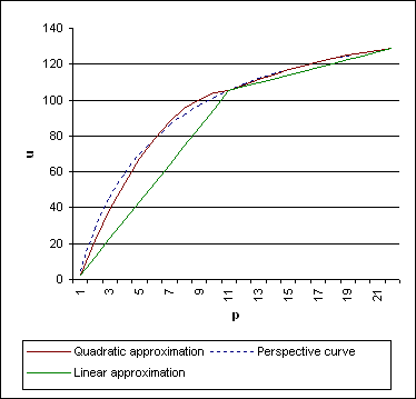
Figure 4:
Figure 4 shows a highly curved hyperbola which is approximated with two consecutive parabolas. The figure shows that one part of a hyperbola is easier approximated by a parabola than another part. That being so, an adaptive span length selection is more effective than a fixed maximum span length. More concretely, if you base the span length on the curvature of the segment of the hyperbola that you try to approximate, you get short spans where needed and long spans where possible: a compromise with a good overall approximation and a small number of spans per scan line.
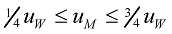
Instead of devising some measure of curvature of a hyperbola section, I use a measure that I already have at hand: the parabola parameter A defines the curvarture of the parabola that we use to approximate the hyperbola. A high (absolute) value of A means a very curved parabola, thereby undoubtedly a bad approximation, and therefore a span that should be subdivided. Earlier I presented an analysis to avoid overshoot. The proposed solution put a low and a high bound on the middle point —what it achieved by this was to reduce the curvature of the parabola in critical situations. For the purpose of span subdivision, we can use exactly the same technique, but with stricter bounds. To avoid overshoot, uM must be between 1/4 uW and 3/4 uW. To avoid excessively curved parabolic spans we might decide that for every span uM must be between 5/16 uW and 11/16 uW; if not, it will be subdivided. This scheme, when applied recursively, automatically avoids overshoot. In addition, it fits a MIP-mapping scheme.
The discontinuities between two consecutive quadratic curves are less severe that those of two consecutive line segments of the same length. For longer spans, the severity of discontinuities depends on the curvature of two consecutive quadratic curves. Discontinuities between two consecutive spans can be "smoothened" by manipulating the control points uM and uW. Moving uM slightly toward uW/2 and uW toward the final end point (of the last span), decreases the discontinuity considerably. Adjusting the positions of the control points by as little as 2% is usually sufficient. Note that discontinuities between two consecutive spans appear when the curvature of at least one of the spans is strong, and that at the same time a strongly curved parabola deviates from the desired (hyperbola) curve. Therefore, an adaptive span-subdivision that is based on a maximum curvature criterion automatically avoids (severe) discontinuities.
Smooth quadtratic projection
In the article "Image scaling with Bresenham", I improved the quality of image interpolation by averaging a pixel with its neighbour when the calculated error exceeds a threshold, and we can adjust the quadratic projection in a similar way. The standard Bresenham algorithm uses an "error" threshold with the accumulated fractional part of the increment value. The "fraction arithmetic" presented here is the same thing by another name. The "Smooth Bresenham" algorithm from the "Image scaling with Bresenham" article introduced a second threshold for which to start averaging, and set it to half of the error threshold. A follow-up online paper refines the approach with an adaptive threshold.
The image scaling algorithm is two-pass: first scale pixels on each scan line horizontally, then scale scan lines vertically. The quadratic image projection algorithm is moves both horizontally and vertically through the source image in a single loop. As a result, the algorithm not only needs to decide whether to average, but also which averaging candidate to select: right, down, or (diagonally) right+down.
When you average a pixel with the next one, you must make sure that there is one more pixel to the right or downwards. You cannot average the pixel at the right edge of the source image with the pixel one beyond the edge. The "Image scaling with Bresenham" article derived a simple criterion to stop averaging before reaching the right or bottom edges —without explicitly testing for these edges in the inner loop. For the quadratic projection, such a criterion is not as simple to find. A practical alternative is to add one extra column and one extra row to the source image, so that there always is a next pixel to average with.
Pseudo-code for the "smooth quadratic projection" algorithm is below. Upon comparison with the earlier pseudo-code for "coarse" projecting, the new part is the series of "IF" instructions that check the "u" and "v" values against thresholds. The "average" function calculates the mean colour of two input colours (see the on-line article "Quick colour averaging" for details), and the "fractional" function returns the fractional part of a value. As can be seen, if both the horizontal and vertical coordinates ("u" and "v") exceed their respective thresholds, the current pixel is averaged with the one that is diagonally to the right and below; if only one coordinate exceeds its threshold, the averaging is horizontal or vertical.
calculate y_start and y_end
LOOP y' FROM y_start TO y_end
    calculate x_start and x_end
    calculate du, ddu, dv and ddv
    calculate threshold_u and threshold_v
    LOOP x' FROM x_start TO x_end
        pix = sourceimage[integer(u), integer(v)]
        IF fractional(u) > threshold_u AND fractional(v) > threshold_v THEN
          pix = average(pix, sourceimage[integer(u) + 1, integer(v) + 1]
        ELSEIF fractional(u) > threshold_u
          pix = average(pix, sourceimage[integer(u) + 1, integer(v)]
        ELSEIF fractional(V) > threshold_v
          pix = average(pix, sourceimage[integer(u), integer(v) + 1]
        END IF
        displaybuffer[x', y'] = pix
        x' = x' + 1
        u  = u + du
        v  = v + dv
        du = du + ddu
        dv = dv + ddv
    END LOOP
    y' = y' + 1
END LOOP
I suggest that you calculate the averaging thresholds per span and separately for the horizontal and vertical directions. Basing the thresholds on the overall horizontal/vertical scale ratio of a span, with the same adaptive criterion as those for Smooth Bresenham, is simple and adequate. For completeness, I give the equations below (but see the errata notes for the article "Image Scaling with Bresenham" for details and background):
pW >= uW ¦ thresholdu = pW - 3 2(pW - uW) pW < uW ¦ thresholdu = pW + 1 · (pW - uW) The thresholdu must be clamped to a low bound of 0.5 (it never exceeds 1.0).
The same calculations apply to thresholdv as well (replace uW by vW).
End notes
Listing 2 implements a demo program that loads a True Color image (in BMP file format) and lets the user rotate it over the horizontal and the vertical axes. The program uses the function ParScanline from listing 1 and the simple (minimal) vector library in listing 3 that defines the dot and the cross products, plus the ability to scale a vector to a unit vector.
This is by far not the first attempt at quadratic interpolation using a Bresenham-like algorithm. However, this article provides an analysis and fixes for several problems and shortcomings that have been attributed with quadratic Bresenham, foremost bad approximation of the perspective foreshortening curve and overshoot. Overshoot was handled rigorously in this article by adding a simple bounds criterion to one of the parabola parameters. The approximation was addressed by selecting a better mid-point parameter for the quadratic equation. I also gave arguments why accuracy should not be overrated. Finally, the exact fraction arithmetic (according to Bresenham) eliminates accumulated round-off errors.
Although I addressed performance issues, the implementation is more suited for exposing the algorithm than for production code. In particular, you might want to replace the calls to the inline functions in the inner loop of the ParScanline function by preprocessor macros, to avoid the overhead of "calling" and inline function (see the article "Winning the Passing Game"). Also, one can remove the "if" statement in the Add method of the Fractional class, which is used four times in the inner loop, with a bit of binary magic on two's complement values. The biggest bottleneck in the demo program is the bitblt function, which is called for every scan line. A better approach is to build the complete projected image in memory and then bitblt only once.
References
- Foley, James D. [et al.]; "Computer Graphics: Principles and Practice"; Addison-Wesley; second edition, 1990; ISBN 0-201-121107.
- In section 19.2.6, this encyclopedic book contains a description of an algorithm that plots conic sections using a Bresenham-like algorithm. The implementation is incomplete and it can only cope with integer values for the parameters of the conic equation.
- Fomitchev, Max; "Winning the Passing Game"; Dr. Dobb's Journal Online Column; 2001.
- When "calling" an inline function, the parameters to the inline function are still passed via the stack. The stack maintenance may cause inline functions to be quite slow in comparison with the preprocessor macros that they meant to replace. The article is available on the Dr. Dobb's Journal web site at http://www.ddj.com/columns/optimize/.
- Hecker, Chris; "Perspective Texture Mapping, Part 4: Approximations" (Behind the Screen); Game Developer; December/January 1995/1996.
- This fourth column from a series on perspective texture mapping discusses three approximations of the perspective foreshortening curve, one of which is the quadratic curve.
- Riemersma, Thiadmer; "Image scaling with Bresenham"; Dr. Dobb's Journal; May 2002.
- A describtion of the "smooth Bresenham" algorithm, which combines the speed of nearest neighbour scaling with a quality that is equivalent to bilinear interpolation.
- Riemersma, Thiadmer; "Image Scaling with Bresenham - Errata"; April 2002.
- Corrections and additions to the article published in Dr. Dobb's Journal. This article is only available on-line.
- Riemersma, Thiadmer; "Quick colour averaging"; Februari 2002.
- Using "bit magic" and tricks of two's completement arithmetic to calculate the average of two three-channels colours on a single operation (that is, without decomposing the colour in three channels first and regrouping them later). This article is only available on-line.
- Smith, Alvy R.; "Incremental Rendering of Textures in Perspective"; SIGGRAPH '80 Tutorial Notes; October 28, 1979.
- The paper gives an analysis of perspective texture mapping, and it develops an incremental algorithm to do so (the incremental algorithm developed in the paper requires floating point arithmetic and a few multiplies plus one divide per pixel). The paper also argues, on theoretical grounds, that approximating the perspective projection by a polynomial (such as a parabola) cannot be sufficiently accurate. The paper is available from Dr. Smith's homepage.
