

Riemersma dither
Dithering along a Hilbert curve with restricted error proliferation
An introductory article of the proposed dither technique, entitled "A Balanced Dither Algorithm", was published in the December 1998 issue of C/C++ User's Journal (now available on-line courtesy of Dr. Dobb's Journal). That article was derived from an earlier version of this page. Since the basic operation and properties of Riemersma dither were better laid out in the C/C++ User's Journal article, this page focuses more on the more technical aspects of the dither algorithm.
Riemersma dither is a novel dithering algorithm that can reduce a grey scale or colour image to any colour map (also called a palette) and that restricts the influence of a dithered pixel to a small area around it. It thereby combines the advantages of ordered dither and error diffusion dither. Applications for the new algorithm would be image processing systems using quadtrees and animation file formats that support palette files (especially if those animation file formats use some kind of delta-frame encoding).
The ordered dither and error diffusion dither algorithms both have their advantages and disadvantages. The advantage of error diffusion over ordered dither is that it can choose colours from any colour map. When you reduce a full colour image to palette colour (with 256 colours), you will want to create an optimal palette for the image for best quality. The error diffusion dither algorithm can use such a palette, but the ordered dither algorithm can only dither to colours from a special "uniform" palette (more on this below). Ordered this has the advantage that the dithering of one pixel does not influence the dithering of surrounding pixels; that is, the dither is "localized". This is especially useful when the dithered image is used in an animation sequence.
Comparing Riemersma Dither with Error Diffusion and Ordered Dither
Before diving into the design and implementation of Riemersma dither, comparing it with the previously mentioned other dither techniques may clarify the concepts. It also allows us to discuss various trade-offs of the different dither techniques. By the way, for most of the following discussion I will assume that we are given a gray-scale image with shades of gray between intensity levels 0 and 255 (for black to white respectively), and that we are dithering the image to a bilevel, black & white image.
Ordered dither algorithms use a fixed matrix; two common approaches are "clustered dot ordered dither" and "dispersed dot ordered dither". The halftoning procedure used in newspapers is an example of clustered dot dither.
The ordered dither algorithm compares the gray level of a pixel to a level in a dither matrix. Depending on this comparison, the pixel is set to either black or white. The matrix contains threshold values between 0 and 255. The size of the matrix and the arrangement of the values have an important effect on the dither process. When a picture is larger than the dither matrix (and it usually is), the matrix is tiled over the image. Every pixel in the source image is compared to only one level in the dither matrix. Neighboring pixels have no effect on the dither result. The book "Digital Halftoning" goes into details of constructing a matrix.
The ordered dither algorithm is easily extended to colour output: just split the input colour into its RGB components and run each component through the dither matrix. Similarly, if the output device can support one extra level of gray between black and white (so the output device supports gray levels 0, 128 and 255), the dither algorithm can first determine the upper and lower bounds of each input pixel and then use a dither matrix to choose between either. That is, a source pixel below 128 is dithered to either 0 or 128 and a source pixel above 128 is dithered to either 128 or 255.
When the ordered dither is extended both to multiple levels and to colour output, this only works if the colour components of the source pixels can be independently dithered. In other words, you split each source pixel into its Red, Green and Blue values, you dither these separately and then you assemble the (dithered) components to a new pixel; assuming that the colour map contains an entry that matches the assembled pixel. In short: this works only if the palette has been carefully laid out to contain the entries that match every possible combination of the levels in the independent Red, Green and Blue matrices. Such a palette is called a "uniform colour map". Uniform colour maps usually are constructed as (linear) RGB cubes, and, hence, they are far inferior to optimized palettes. (See the article "A gamma-corrected uniform palette" for a minor improvement on linear uniform palettes.)
Error diffusion dither algorithms spread the error (caused by quantizing a pixel) over neighboring pixels; the best known example of error diffusion dither is the "Floyd Steinberg" dither.
In error diffusion, the value of a pixel is compared to a single threshold of 50% gray (that is, when black is 0 and white is 255, each pixel is compared to 128). The pixel is set to either black or white, based on that comparison. After outputting the dithered pixel, the algorithm calculates the difference between the source pixel and the output pixel (a simple subtraction), and then it spreads this difference (the "error") over neighboring pixels. In other words, the algorithm changes the source image as it goes through it. The error is partitioned between pixels to the right of the current pixel and pixels below the current pixel. The "diffusion" part of the error diffusion algorithm is thus two-dimensional.
Error diffusion is trivially extended to both colour images and to multiple output levels. For every source pixel, you still search the closest entry in the colour map (i.e., the entry in the palette for which the "error" is the smallest). In case of colour output, you split the error into the RGB components and you spread these error components to the neighbouring pixels. The error diffusion algorithm can work with optimized colour maps, because the source pixels are not split into components and reassembled; only the quantization error is partitioned.
Desirable properties of a dither are:
- The ability to use an optimal (non-uniform) colour map (palette).
- The effect of dithering one pixel should not influence neighbouring pixels.
- In the spatial domain, the dithered image should not have visible dither patterns.
- In the frequency domain, the dither should spread the error in the high frequencies (which are less visible than the low frequencies).
The support for optimal colour maps has already been discussed in the preceding paragraphs. In my opinion, the visual quality that one gains by using an optimized palette is often underestimated. Riemersma dither supports optimal colour maps in a similar way as error diffusion algorithms.
The ordered dither algorithm is a "point process". The value to which a pixel is quantized depends only on the pixel colour and its position. With error diffusion dithers, on the other hand, the dither result of any pixel also depends on the dither results of its neighboring pixels. This means that modifying one pixel in the source image can provoke changes in a large area of the dithered result. Riemermsa dither is an "area process": the quantization of one pixel influences a limited number (typically 16) of neighbouring pixels.
Ordered dither shows strong patterns, which degrade the subjective quality of a dithered picture. Error diffusion dithers suffer from a "directional emphasis", which are not as disturbing as the ordered patterns but which are quite visible nonetheless. Many texts on implementing the error diffusion algorithms propose simple adjustments to remove the "directional emphasis" as much as possible (in his book "Digital Halftoning", Robert Ulichney proposes to use a serpentine raster and adding a small amount of white noise to the source image prior to dithering). Although there is still only little experience with Riemersma, it appears that Riemersma dither is free from both patterning and "directional emphasis" (both due to the use of a space filling curve).
The error diffusion dither algorithms score quite well on the criterion to dither primarily in the "high frequencies", which makes the dithered pictures more detailed and more attractive (see "Digital Halftoning", page 236). Ordered dither is coarser than error diffusion, due to the presence of low frequencies. Riemersma dither scales somewhere between the two (it is coarser than error diffusion).
The Riemersma dither algorithm presented here is a compromise: it is an "area process" instead of a "point process" and the produced dither is coarser than that of the error diffusion algorithm. On the positive side is that it can use any colour map (especially optimal colour maps) and that it is free from patterning and "directional emphasis". Riemersma dither was developed with frame animation in mind. As such, the "area process" attribute is important, because it can dramatically reduce the size of the delta between one frame and the next.
For a visual comparison of the discussed dither algorithms, below is the well known picture of Lena: once as a JPEG file (RGB, and undithered) and three times as a dithered image. To compare the four images, you should set the display to an RGB mode, because the pictures use optimized palettes, and make sure that your browser does not enforce some "web-safe" palette. You can also save the images and examine them with a picture viewer of your choosing.
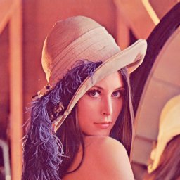 Original picture (RGB) |
 Ordered dither, uniform palette |
 Floyd-Steinberg dither (error diffusion), optimized palette |
 Riemersma dither, optimized palette |
Dithering along a Hilbert curve
The first step towards a dither procedure that combines localized dither and optimized colour mapping is to reduce the error diffusion algorithm to its bare essentials. Error diffusion works by adding the difference between a pixel in the source image and the resulting mapped pixel to a set of neighboring pixels. I reduced this set pixels to a single pixel. Normally, the error diffusion algorithm spreads the error (the difference between the source pixel and the mapped pixel) both horizontally and vertically, but if you only have one pixel to carry the error to, the algorithm implicitly becomes one-dimensional.
I mention the one-dimensional nature of the simplified error diffusion algorithm, because the next step is to align the algorithm to a Hilbert curve. The Hilbert curve is a "space filling curve", it is a kind of fractal that runs through a square grid and visits every grid point exactly once without intersecting itself. By applying this uni-dimensional algorithm to a Hilbert curve, I have obtained a very simple, but effective way to dither a two-dimensional picture.
 The forwarded error that was mentioned in the previous paragraphs holds
the accumulated total of all quantization errors. This accumulated error is
added to the value of a pixel prior to quantizing it. For example, when
dithering a gray level image to black and white, every pixel is mapped to
either black (level 0) or white (level 255) and the error introduced by this
mapping is in the range -127..128 for every pixel (this is the quantization
error). The single error accumulator is the sum of the quantization errors of
all pixels that were quantized so far.
The forwarded error that was mentioned in the previous paragraphs holds
the accumulated total of all quantization errors. This accumulated error is
added to the value of a pixel prior to quantizing it. For example, when
dithering a gray level image to black and white, every pixel is mapped to
either black (level 0) or white (level 255) and the error introduced by this
mapping is in the range -127..128 for every pixel (this is the quantization
error). The single error accumulator is the sum of the quantization errors of
all pixels that were quantized so far.
The image (on the right) is again the "Lena" picture dithered with the Hilbert curve and the error proliferation as described above. The picture was dithered to black & white to better display the artefacts introduced by the dither algorithm.
Although I have simplified the error diffusion algorithm, a change in
a pixel near the start of the image may still affect, through the error
accumulator, the quantized values of a large number of subsequent pixels.
Reducing the error proliferation
Restricting the number of surrounding pixels that the quantization error for a pixel affects is simple in concept. Instead of adding the accumulated error of all previous pixels to the current pixel before quantizing it, you just add to the pixel the accumulated error of the last, say, 16 pixels. In other words, you keep a list of the quantization errors of a number of recent pixels. At every new pixel to quantize, to add to the pixel value all the quantization errors in the list. Then you quantize the pixel. This creates a new quantization error (for the pixel just quantized). This error is added to the list, while removing the oldest error entry from the list.There is a pitfall in this scheme: when removing an entry from the quantization error list, you are effectively adding a bias of the negative value of the removed entry to the list.
An example will make this clearer. Assume that you keep a list of 4 most recent quantization errors. When dithering a gray surface (gray value 128) to black and white, the progression would be:
| quantization error list | source pixel | adjusted pixel | quantized pixel | |||
|---|---|---|---|---|---|---|
| 0 | 0 | 0 | 0 | 128 | 128 | 255 |
| 0 | 0 | 0 | -127 | 128 | 1 | 0 |
| 0 | 0 | -127 | 128 | 128 | 129 | 255 |
| 0 | -127 | 128 | -127 | 128 | 2 | 0 |
| -127 | 128 | -127 | 128 | 128 | 130 | 255 |
| 128 | -127 | 128 | -127 | 128 | 130 | 255 |
Notes about the construction of the table:
- The "adjusted pixel" value is the source pixel plus all values in the "quantization error list".
- The adjusted pixel is mapped to either 0 or 255, whichever is closest. This becomes the "quantized pixel" result.
- The difference between the source pixel and the quantized pixel becomes the new (rightmost) entry in the quantization error list on the next row.
- Gray level 128 is slightly above the mid-level between 0 and 255. That is why the adjusted pixel is slowly incrementing in the first five rows.
On the sixth line, the leftmost value was dropped from the list. The accumulated error of the list is suddenly 127 higher than what it should have been. Dropping the oldest entry from the root creates a severe error in the dithered result.
In the quantization error list of the above example, all entries have the same weight. The solution to the problem of the "bias" introduced by dropping a value from the list is to give the old entries in the quantization error list a (much) smaller weight than the new entries. As an entry moves down from the top of the list towards the bottom, its weight gradually lowers. An exponentially decaying curve works well in my experience.
First, you need to choose the ratio of the highest weight versus the lowest weight. The length of the quantization error list is another parameter that you must select. When the ratio is r and the list length is q, then the base value for the exponential curve is:

![list[i] = 1/r * pow(b, i)](./images/hilbert4.gif)
The following table is a same example, but now the four values have a weight attached to them. The oldest entry has the weight of 1/4th of the newest entry.
| quantization error list | source pixel | adjusted pixel | quantized pixel | |||
|---|---|---|---|---|---|---|
| 0 | 0 | 0 | 0 | 128 | 128 | 255 |
| 0 | 0 | 0 | -127 | 128 | 1 | 0 |
| 0 | 0 | -127 | 128 | 128 | 176 | 255 |
| 0 | -127 | 128 | -127 | 128 | 30 | 0 |
| -127 | 128 | -127 | 128 | 128 | 195 | 255 |
| 128 | -127 | 128 | -127 | 128 | 63 | 0 |
| weights | ||||||
| 0.25 | 0.40 | 0.63 | 1.0 | |||
The resulting dither pattern in the last table is what we would expect for the dither pattern for mid-level gray. Note that the quantization error list is much too short to achieve a decent dither quality. I regard an error list of 16 as a minimum. In my own implementation, I have also set the weight ratio of the oldest entry versus the newest entry to 1:16 (instead of to 1:4 as in the above table).
Other space filling curves
The Hilbert curve is a simple curve that has a high coherence of neighbouring pixels. Relating to dithering alogn the path of a space filling curve, the high coherence of neigbouring pixels means that the quantization error in each pixel is spread foremost over its closely surrounding neighbours. This is obviously a good property, because it keeps the quantization errors from "bleeding" into remote surroundings of the pixel.
As a general purpose curve, the Hilbert curve is the best choice. For any specific image, however, one can often create a curve that is optimal for that picture. Such curves are called "context-based space filling curves", see the paper by Dafner et al. for an example. Using a context based curve might improve the image quality of the dither, and especially its perceived sharpness, due to higher coherence of neighbouring pixels.
However, for the purposes of animation and image compression, it is disadvantageous to use a different space filling curve for each image or frame. First of all, the you may need to store the space filling curve. Secondly, different space filling curves could generate large differences in successive frames. Both of these aspects depend on how the image is stored and, of course, on how much the curves of two successive frames change.
Example program
A simple example program in C that created the dithered "Lena" (black & white) picture on this page implements the concepts of this article. It was tested with Borland C++ for DOS in large memory model, but I have tried to avoid non-portable constructs. The bulk of the code deals with the Hilbert curve generation. The implementation of the error proliferation is straightforward.
Conclusion
Although this paper focuses on dithering to black and white, the same principles apply to the case where intermediate gray levels are available. In a similar vein, the algorithm can be adapted to colour images (and restricted colour maps) by keeping three quantization error lists, for each of the red, green and blue channels.
Dithering along a space filling curve is a relatively young object of study. I expect that the results of the simple dither that I have presented here can be adjusted and improved, for example:
- by using a different space filling curve, like Peano or Sierpinsky,
- by adjusting the decay speed and the length of the quantization error list,
- by substituting the exponential decaying weights by a different curve.
Related to dithering are the topics of computing the best colour map (creating an optimal palette) and of doing the quantization step as accurately as possible.
References
- Dafner, R., D. Cohen-Or and Y. Matias; "Context-based Space Filling Curves"; Computer Graphics Forum; volume 19, issue 3 (August 2000).
- This article presents a simple algorithm to generate a space-filling curve by merging blocks of 2×2 pixels. The selection of which blocks to combine, in what order, is based on a user-defined "weight" function. By making the weight function a function of the pixel coherence of the blocks, this allows one to generate a space-filling curve with optimal coherence for a particular picture.
- Gosselink, Pieter; "Gosselink Dither"; Dr. Dobb's Journal; volume 19, issue 15 (December 1994).
- Gosselink dither combines ordered dither and error diffusion by creating a large set of square tiles, one for each possible colour in an RGB cube. Each tile is then dithered using a simplified error diffusion algorithm. The dithered tiles are used as ordered dither matrices, where the RGB indices of each pixel in the original picture select the tile to use. The memory requirements of Gosselink dither are steep.
- Riemersma, Thiadmer; "A Balanced Dither Algorithm"; C/C++ Users Journal; volume 16, issue 12 (December 1998).
- The article derived from this WWW page contains more introductary material plus discussions of the ordered dither and the error diffusion dither algorithms.
- Ulichney, Robert; "Digital Halftoning"; The MIT Press; 1987.
- An overview and discussion of various dithering and halftoning
algorithms. The book is becoming somewhat outdated: new error diffusion
matrices like Burkes and Sierra are absent from the book, and the research
on dithering using space-filling curves is also missing.
The book may be out of print, but Dr. Dobb's Journal publishes a CD-ROM that contains Ulichney's book in electronic form.
